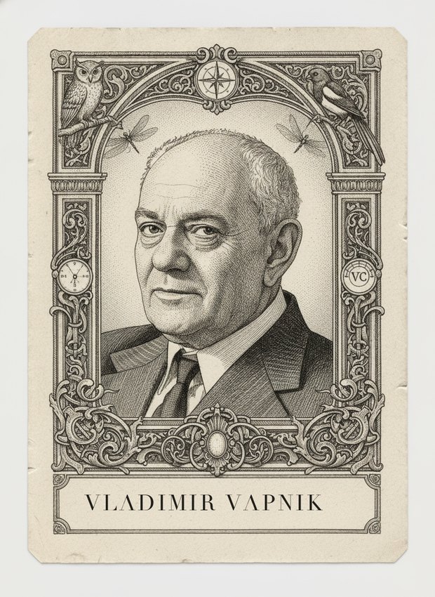
Vladimir Vapnik

Life and career

Vladimir Naumovich Vapnik was born in 1936 in the Soviet Union, and the arc of his career is inseparable from the fact that Soviet and Western machine learning developed for thirty years in near-total isolation from each other. He was educated in mathematics — undergraduate work at Samarkand State University in Uzbekistan, then a doctorate in Moscow — and in 1961 joined the Institute of Control Sciences of the Soviet Academy of Sciences, where he spent roughly three decades and headed the computer science research department.

It was there, in collaboration with Alexey Chervonenkis, that he built the theory that bears both their names. Beginning in the mid-1960s, the two produced a sequence of papers on uniform convergence of empirical frequencies to their probabilities, culminating in the results the West would rediscover, translate, and eventually build an entire theoretical subfield on. The Soviet work on pattern recognition in that era was often more mathematically rigorous than its Western counterparts, and considerably less known. Vapnik's books — *Estimation of Dependences Based on Empirical Data*, published in Russian in 1979 and in English in 1982 — were the channel through which some of it leaked out.

In 1990 Vapnik left for the United States and joined AT&T Bell Laboratories in Holmdel, New Jersey, entering what was then arguably the most productive machine learning group in the world: Yann LeCun, Isabelle Guyon, Bernhard Boser, Corinna Cortes, Patrice Simard, and others, working on handwritten digit recognition for check reading with real accuracy targets and real data. The confrontation between Vapnik's theory and the group's engineering culture produced the support vector machine almost immediately. Boser, Guyon, and Vapnik presented the optimal margin classifier in 1992; Cortes and Vapnik published the soft-margin extension in 1995. In the same year Vapnik published *The Nature of Statistical Learning Theory*, the book that carried VC theory to a broad audience, followed by the more technical *Statistical Learning Theory* in 1998.

He remained in industrial research for the rest of his career — NEC Laboratories America in Princeton, later Facebook AI Research — with academic affiliations in London and New York. He is known for a genuine and frequently repeated aphorism, borrowed from Kurt Lewin and made his own: "Nothing is more practical than a good theory." He is also known, less comfortably for parts of the field, for his sustained skepticism toward deep learning — his position being that stacking layers and tuning empirically is engineering without a theory of why it should generalize. His later research program, on learning using privileged information and on what he has called the "complete statistical theory of learning," reflects a continued insistence that learning should be understood, not merely achieved.

Vapnik has received the Kolmogorov Medal, the IEEE Frank Rosenblatt Award, the Benjamin Franklin Medal, and election to the U.S. National Academy of Engineering, among other honors.

Key contributions

**VC theory.** The question Vapnik and Chervonenkis answered is the foundational one: under what conditions does minimizing error on a training sample control error on unseen data? Their answer replaces counting parameters with measuring the *capacity* of a hypothesis class. A class H shatters a set of n points if it can realize all 2ⁿ labelings of them; the VC dimension of H is the size of the largest set it shatters. The Vapnik–Chervonenkis theorem gives, with probability at least 1 − δ over the draw of the sample, a bound of the form

R(h) ≤ R̂(h) + O( sqrt( (d (log(2n/d) + 1) + log(4/δ)) / n ) )

uniformly over all h ∈ H, where d is the VC dimension. Three features are worth dwelling on. The bound is *uniform* over the class, which is what makes it apply to the hypothesis you selected by looking at the data. It is *distribution-free* — it holds for every data distribution. And it is driven by d, not by the number of parameters or the ambient dimension, which is why a class with infinitely many parameters can still generalize and a class with three parameters can fail to. The Vapnik–Chervonenkis–Sauer–Shelah lemma, bounding the growth function polynomially once d is finite, is the combinatorial engine underneath.

**Structural risk minimization.** The bound is not merely descriptive; it is a design principle. Order candidate hypothesis classes H₁ ⊂ H₂ ⊂ … by increasing capacity, and choose not the class that fits best but the class minimizing the *sum* of empirical risk and the capacity term. This is a fundamentally different philosophy from AIC or BIC: it is finite-sample, distribution-free, and worst-case rather than asymptotic and average-case. It is also the intellectual ancestor of essentially every modern generalization bound — Rademacher complexity, PAC-Bayes, margin bounds, stability bounds.

**The support vector machine.** Given linearly separable data, infinitely many separating hyperplanes exist; VC theory says pick the one that minimizes capacity, and Vapnik showed that for the class of hyperplanes with margin γ separating data of radius R, the effective VC dimension is bounded by roughly R²/γ² — *independent of the ambient dimension*. So maximize the margin. The resulting quadratic program has a dual whose solution depends on the training data only through inner products, and whose solution is supported on the small subset of points lying on the margin — the support vectors. Two extensions completed the method: the kernel trick, replacing inner products with a Mercer kernel K(x, x′) to obtain a linear separator in an implicit high-dimensional feature space at no extra cost (this is how an SVM solves XOR), and the soft margin of Cortes and Vapnik, introducing slack variables with a cost parameter C so that non-separable and noisy data are handled by trading margin against violations. Support vector regression with the ε-insensitive loss followed.

**Transduction and related programs.** Vapnik argued repeatedly against solving a harder problem than necessary: if you only need labels for a specific finite test set, estimate those directly rather than inducing a function over the whole input space. Transductive SVMs and his later work on learning using privileged information — where extra information available at training time but not at test time is used to shape the learning problem — both follow from that principle.

In battle

Vapnik's computed profile is one of the strongest and broadest on the roster: mean 36.6 over 101 problems, seven dominant scores at 80 or above, and fifteen at 70 or above. He is not a single-formula specialist; he carries a large fraction of the supervised-learning problem space.

His category strengths tell the story immediately. Small-sample sits at **86** — by a wide margin the highest category score in his profile, and the reason is structural: VC bounds are finite-sample and distribution-free, so they are the right tool precisely when n is small and asymptotics are worthless. Classification follows at 58 across seventeen problems, computability at 56, testing at 54.

His peak is **P023 — The line between two clouds** (98), which the judge describes as a restatement of his life's work — separable clouds in thirty dimensions in a 1990s setting, with a demand that the generalization guarantee be a theorem rather than an empirical hope. That is the optimal-margin classifier of Boser, Guyon, and Vapnik exactly. **P032 — What can be learned at all?** (92) is learnability theory itself, the question VC dimension was invented to answer. **P110 — Fifty examples in the test set** (88) rewards his finite-sample machinery where anyone reasoning asymptotically has nothing to say. **P025 — Sixty thousand digits** (86) is MNIST, the actual Bell Labs problem he worked on, and where SVMs were competitive with the best neural networks of the era. **P024 — XOR** (84) is the kernel trick's canonical demonstration. **P005 — Prediction intervals without a model** (84) reflects distribution-free reasoning; **P027 — Classify with 30 labels and 30,000 unlabeled** (80) and **P028 — Which examples deserve labels?** (79) draw on transduction and on margin-based active learning.

The losses are clean and clarifying. He scores 5 on **P248 — The machine that overdosed** — the Therac-25 race condition — because concurrency verification in safety-critical device software shares no machinery with statistical generalization theory. **P183 — Cool it slowly** (8) is simulated annealing, **P190 — Sequence the robot's actions** (10) is planning, and **P185 — Optimize across the datacenter** (10) is large-scale systems optimization; his optimization average is 22.4, which surprises students who think of him as an optimization person. He is not: he formulates convex programs and hands them to solvers, which is a different skill from designing algorithms for combinatorial and stochastic search. **P167 — How few bits for a good-enough picture** (10) is rate–distortion, information theory that is not his (information: 20). And **P143 — The coefficient that flips sign** (7) is a causal-confounding problem — the sign-flip under conditioning is Simpson's-paradox territory, and Vapnik's framework has no notion of an intervention at all. His entire theory is about a fixed unknown distribution P(x, y) and generalization to new draws from it; change the distribution deliberately and the guarantees say nothing.

The strategic reading: Vapnik is a premium pick for any classification problem, and an especially devastating one when the sample is small, the dimension is high, and the problem asks for a *guarantee* rather than a benchmark number. He weakens on perception and NLP at modern scale — the deep learning era he has publicly resisted — and collapses entirely on systems engineering, search, planning, and causal identification.