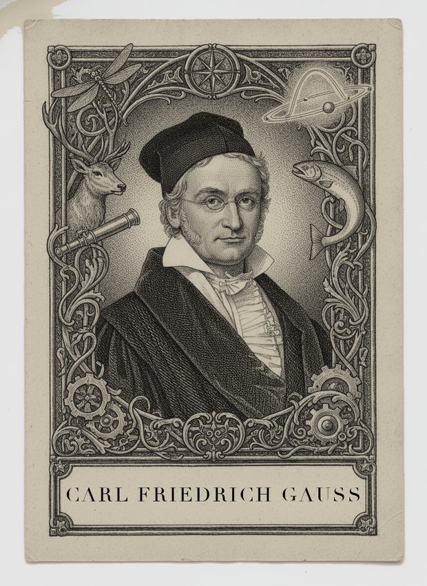
Carl Friedrich Gauss

Life and career

The stories about Gauss's precocity are so numerous that it is tempting to discount them, but the outline is not in dispute. He was born in 1777 in Brunswick to a poor family — his father a gardener and bricklayer's assistant, his mother barely literate — and his mathematical talent was conspicuous early enough that the Duke of Brunswick undertook to fund his education. The most-repeated anecdote has a schoolmaster setting the class to sum the integers from 1 to 100 as busywork, and the young Gauss producing the answer almost immediately by pairing terms from the ends inward. Whether the details are exactly right, the pattern is: Gauss's characteristic move throughout his life was to find the structural shortcut that made brute labor unnecessary — and then, often, to do the brute labor anyway, faster than anyone else.

He studied at the Collegium Carolinum and at Göttingen, and as a teenager proved that a regular 17-sided polygon is constructible with compass and straightedge — the first advance on the Greek constructibility problem in two millennia, and the result that decided him on mathematics over philology. At twenty-one he completed the *Disquisitiones Arithmeticae* (published 1801), which essentially founded modern number theory as a systematic discipline: congruences, quadratic reciprocity, the theory of forms. It is one of the few books in mathematics that can reasonably be said to have created its field.

His public fame, though, came from astronomy. On the first day of 1801 the Italian astronomer Giuseppe Piazzi observed a new object — the asteroid Ceres — tracked it for a few weeks, and then lost it in the sun's glare. There was not enough data, by the methods of the day, to predict where it would reappear. Gauss, then twenty-four, developed an orbit-determination method that extracted a full elliptical orbit from the sparse observations and predicted where to look. Ceres was recovered near his prediction. It was a spectacular, public, unambiguous vindication of computational method over guesswork, and it made him famous outside mathematics.

In 1807 he became professor of astronomy and director of the observatory at Göttingen, a post he held for the rest of his life. He was not a natural teacher and did not enjoy lecturing, though he supervised a remarkable set of students including Dedekind and Riemann. His personal life was marked by loss — his first wife Johanna died in 1809, and a son shortly after, in a period that also produced *Theoria Motus*. He worked on geodesy for years, personally conducting the survey of the Kingdom of Hanover and inventing the heliotrope to reflect sunlight for long-distance sighting; the differential geometry of *Disquisitiones generales circa superficies curvas*, including his Theorema Egregium on intrinsic curvature, came directly out of the practical problem of measuring a curved Earth. With Wilhelm Weber he built one of the first working electric telegraphs, and did foundational work on magnetism.

His publication habits were a genuine loss to the field. His motto was *pauca sed matura* — few but ripe — and he withheld work he considered unfinished, including substantial results in non-Euclidean geometry, elliptic functions, and complex analysis that others rediscovered and published decades later. He died at Göttingen in 1855.

Key contributions

For a data-science audience, three of Gauss's contributions form the substrate under nearly everything.

**Least squares and its probabilistic justification.** Gauss claimed to have used the method of least squares from about 1795; Legendre published it first, in 1805, and a bitter priority dispute followed. What is not disputed is that Gauss supplied the first *principled reason* for it, in *Theoria Motus Corporum Coelestium* (1809). His argument runs backward from a desideratum: assume that the arithmetic mean is the right estimate of a location parameter from repeated observations, ask what error distribution makes the most probable value coincide with the mean, and derive the normal density as the answer. Then, under that error law, the estimate that maximizes the probability of the observed data is exactly the one minimizing the sum of squared residuals. This is a maximum-likelihood argument more than a century before Fisher named it, and it is the reason the normal distribution is called Gaussian.

He later did better than that. In *Theoria Combinationis Observationum Erroribus Minimis Obnoxiae* (1821–23) he replaced the normality assumption with a squared-error loss criterion and proved what we now call the Gauss–Markov theorem: among all linear unbiased estimators of the coefficients in a linear model, least squares has minimum variance, whatever the shape of the error distribution — requiring only zero mean, constant variance, and uncorrelated errors. That shift, from "least squares is optimal because errors are normal" to "least squares is optimal in a well-defined sense regardless," is the more sophisticated result and the one that matters when you fit a regression to data you have no reason to think is Gaussian.

**Computation.** Gauss was, in a way modern practitioners should appreciate, an algorithms person. Gaussian elimination for solving linear systems is his name attached to a method he systematized for exactly the normal-equation problems least squares generates. He developed iterative refinement schemes for the same purpose (the Gauss–Seidel method descends from this work). And a technique for computing what we would now call the discrete Fourier transform by recursive decomposition appears in his unpublished papers around 1805 — an FFT algorithm predating Cooley and Tukey by a century and a half, unpublished and therefore without influence.

**The normal distribution and error theory as a whole.** Together with Laplace's central limit theorem, Gauss's error analysis produced the standard model that dominated quantitative science for a century: observations equal signal plus independent Gaussian noise, estimate by minimizing squared residuals, propagate uncertainty through the linearized model. Every Kalman filter, every ordinary-least-squares fit, every Gaussian-noise assumption in a probabilistic model, and every bundle-adjustment solver in computer vision is running on this framework.

The limitation is built into the strength. The Gaussian model's tails are extraordinarily thin, and squared-error loss weights a single gross outlier by the square of its deviation. Robust statistics exists because Gauss's framework, applied to data with heavy tails or contamination, fails badly and quietly. He worked with careful astronomical and geodetic measurements where the assumption largely held.

In battle

Gauss's profile is that of a devastating specialist rather than an all-rounder: mean 29.7, median 20, only four problems at 80 or above but fifty at 20 or below. When the problem is estimation from noisy continuous measurements, he is close to unanswerable. Outside that region he falls off a cliff.

His single best score is "Why least squares, exactly?" at 99 — a problem that is, in effect, asking for his own 1809 and 1821 arguments. "Find the lost planet" (98) is Ceres, literally: recovering an orbit from sparse observations, the problem that made his reputation. The surprise on his sheet, and the most instructive part of it, is his perception category average of 88.5, driven by "Rebuild the city from vacation photos" (92) and "Where did every pixel go?" (85). Structure-from-motion and optical flow look like modern computer vision, but underneath they are enormous nonlinear least-squares problems solved by exactly his machinery — normal equations, Gaussian error models, iterative refinement, sparse elimination. A graduate student who has written a bundle adjuster has written Gauss's method with better hardware.

The rest of his strong region follows the same logic. "Why tall fathers have shorter sons" (78) is regression toward the mean, downstream of his linear-model apparatus. "Feed the army for pennies" (75) and "The charge on a single drop" (75) are linear-system solving and careful error analysis of small physical measurements. "Where to place the measurements" (74) is optimal experimental design, which is a variance-minimization question over the design matrix — a direct application of the Gauss–Markov framework. His category averages tell the story cleanly: regression 55.3 across nine problems, small-sample 54.3, high-dimensional 35.8, optimization 29.4 across fifteen.

His failures are sharply patterned. Anything **discrete, combinatorial, or sequential** collapses: "Sequence the robot's actions" (8), "Prune the game tree, provably" (8), "The tournament of strategies" (8), "Learning on the molecule graph" (8). Gauss's mathematics is continuous analysis over the reals; planning, adversarial search, evolutionary game dynamics, and graph-structured learning live in a different register entirely, which is why his games average sits at 16.9 and his networks average at 17.2. **Randomized and worst-case learning theory** also defeats him — "The dice make it learnable" (5) is PAC-style analysis, where the whole point is to avoid the distributional assumptions his framework is built on. And his outright floor is "What happened first?" (5), the problem of establishing causal event ordering across machines with no shared clock: distributed-systems logical time has no bridge to least squares at all, and the profile says so bluntly.

The pedagogically useful reading is that Gauss's weakness is not ignorance but *commitment*. He is the strongest possible embodiment of one modeling stance — continuous parameters, additive well-behaved noise, quadratic loss, exact linear algebra — and that stance is enormously powerful and genuinely narrow. Play him on estimation, regression, calibration, geometry, experimental design, and any problem that reduces to solving a large well-conditioned system. Do not play him on heavy tails, adversaries, discrete structure, distributed coordination, or anything where the difficulty is that you cannot write down a noise model in the first place.