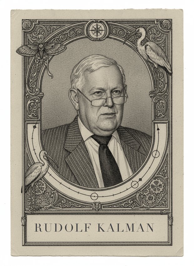
Rudolf Kalman

Life and career

When Apollo 11 fired its engines to leave lunar orbit, the spacecraft's onboard computer knew where it was because of an algorithm published nine years earlier in a mechanical engineering journal that had rejected the author's first attempt at getting it into a more prestigious venue. The algorithm was the Kalman filter, and its inventor was a Hungarian-born engineer whose result was initially met with skepticism by the statisticians whose problem he had solved.

Rudolf Emil Kálmán was born in Budapest in 1930. His family emigrated to the United States during the Second World War, and he did his undergraduate and master's degrees in electrical engineering at MIT, finishing in 1954. His doctorate came from Columbia in 1957, under John Ragazzini, in the then-new area of sampled-data control systems — the mathematics of controlling continuous physical systems with discrete digital measurements, which was becoming urgent precisely because digital computers were arriving.

The critical years were at the Research Institute for Advanced Study (RIAS) in Baltimore, a small privately funded institute where Kalman worked from 1958 to 1964 alongside Solomon Lefschetz and others. It was an unusual place — a research shop attached to the Martin aircraft company, with almost no teaching duties and a mandate to do fundamental mathematics with applications in view. In a compressed span of about three years Kalman published the papers that created modern state-space control theory: the 1960 discrete-time filter, the 1961 continuous-time version with Richard Bucy, and the work establishing controllability and observability as the structural properties of linear systems.

The reception was mixed. Kalman's approach was thoroughly *engineering* in its framing — recursive, computational, expressed in matrices and state vectors rather than in the frequency-domain language then standard — and statisticians noted that Wiener's earlier filtering theory covered related ground. The decisive endorsement came from Stanley Schmidt at NASA Ames, who heard Kalman present the work, saw immediately that it fit the Apollo trajectory estimation problem, and led the team that adapted it into the extended Kalman filter for nonlinear orbital dynamics. Apollo flew with it. So, subsequently, did essentially every guided vehicle built since.

Kalman moved to Stanford (1964–1971), then to the University of Florida, where he founded the Center for Mathematical System Theory, and later held a chair at the Swiss Federal Institute of Technology in Zurich while retaining the Florida position. His later work took a more austere and critical turn: he became a sharp critic of what he saw as sloppy statistical practice in econometrics and elsewhere, pursuing an approach he called "system identification from data without prejudice," insisting that models should be extracted from data by algebraic means rather than imposed by assumption. He was blunt about it, and it made him a somewhat isolated figure in his later career.

He received the IEEE Medal of Honor in 1974, the Kyoto Prize in 1985, and the National Medal of Science in 2009, presented by President Obama. He died in Gainesville, Florida, in 2016.

Key contributions

**The Kalman filter (1960).** Posit a linear dynamical system with Gaussian noise: the hidden state evolves as *x*ₖ = *F x*ₖ₋₁ + *B u*ₖ + *w*ₖ, and you observe *z*ₖ = *H x*ₖ + *v*ₖ, with *w* and *v* zero-mean Gaussian with known covariances *Q* and *R*. The filter maintains a Gaussian belief over the state — a mean and a covariance — and updates it in two alternating steps. **Predict**: push the mean through the dynamics and inflate the covariance by *Q*. **Update**: on receiving a measurement, compute the innovation (the difference between the observation and its prediction), weight it by the Kalman gain *K* = *P Hᵀ*(*H P Hᵀ* + *R*)⁻¹, and correct the mean; then shrink the covariance accordingly.

For a statistically trained reader, three things about this deserve emphasis. First, it is exactly Bayesian inference — the conjugacy of Gaussians under linear maps means the exact posterior stays Gaussian forever, so the filter is not an approximation but the closed-form solution. Second, it is **recursive**: the update depends only on the previous belief and the current measurement, so memory and computation per step are constant regardless of how long the system has been running. In 1960, with kilobytes of memory available, this was the whole ballgame. Third, the Kalman gain is an automatic bias-variance trade: when measurement noise *R* is large the gain is small and the filter trusts its model; when process noise *Q* is large the gain is large and the filter trusts the data. It is adaptive shrinkage, derived rather than tuned.

**Controllability and observability.** Kalman's structural contribution may be more fundamental than the filter. He defined **controllability** — can an input sequence drive the state anywhere in the state space? — and **observability** — can the state be reconstructed from the output history? — and gave algebraic rank conditions on the matrices [*B*, *FB*, *F²B*, …] and [*H*; *HF*; *HF²*; …] that decide each. He then proved the **duality** between them: the observability problem for one system is the controllability problem for its transpose. The Kalman decomposition splits any linear system into controllable/uncontrollable and observable/unobservable subspaces, which tells you what part of a system you can actually do anything about. This turned control from a collection of frequency-domain techniques into linear algebra on state spaces.

**LQG and the separation principle.** Combining the filter with the linear-quadratic regulator gives Linear-Quadratic-Gaussian control, and the accompanying **separation theorem** — that under linear dynamics, Gaussian noise, and quadratic cost, the optimal controller is obtained by estimating the state optimally and then applying the optimal control law *as if* the estimate were the true state. Estimation and control decouple exactly. This is a genuinely surprising result and it does not survive relaxation of the assumptions, which is the source of much of the difficulty in modern partially observed control.

In battle

Kalman is one of the strongest all-around cards in the midcentury cohort: mean 35.2, median 28, nine dominant scores, and only thirty-three problems below 20 — a much broader profile than the symbolic AI figures, because state estimation touches almost anything that moves through time under uncertainty.

His peak is **Balance the broomstick** (P065) at 96. The cart-pole is linearizable about the upright equilibrium, which is precisely where his machinery is sharpest: check controllability of the linearized system, estimate the state from noisy cart-position measurements, feed back through an optimal gain. He owns the entire model-based half of the problem and forfeits the model-free half, since learning to balance from repeated failures was never his question. The same structure explains **Act on what you cannot see** (P230) at 90 — partial observability is the condition the filter was built for — and **The missile and the evader** (P208) at 90, pursuit-evasion, where guidance under noisy tracking is the literal application his employers cared about.

**Depth for a robot on Mars** (P241) at 90 and **Find the lost planet** (P017) at 85 and **Find the lost submarine** (P210) at 83 form a coherent group: fusing noisy observations of a moving or uncertain object into a shrinking uncertainty ellipse is the same computation whether the object is a rover's pose, a planet, or a submarine. **The software that may not fail** (P080) at 82 reflects aerospace-grade reliability engineering, the culture he worked inside. **The trend with a memory** (P138) at 80 is time-series with state — his state-space formulation subsumes ARIMA models, and the modern structural time-series literature runs on Kalman recursions.

His category means are worth reading closely because they are unusual. `regression` 73.3, `causality` 69.5, `perception` 66.0, and `rl` 50.1 across eighteen problems are all high — the reinforcement learning number in particular, because optimal control is RL's other parent and the LQR is the one control problem with a clean closed-form optimal policy. He is a genuinely quantitative figure with a real probabilistic model, unlike most of his midcentury peers.

Where he fails, he fails for a specific reason: no discrete structure, no symbols, no combinatorics. He scores 10 on **Search deep on a shoestring of memory** (P193, iterative deepening) and 10 on **Let the machine find the proof** (P195), 9 on **Small tools, loosely joined** (P246, the Unix philosophy), 8 on **A thousand categories** (P148, ImageNet-scale classification) and 8 on **The variable you removed is still there** (P289, proxy variables in fairness), and 5 on **Find the needle documents** (P084, TF-IDF retrieval) — his floor, and a total mismatch: nothing in state-space estimation touches corpus statistics or relevance ranking. `classification` at 9.0 and `nlp` at 10.5 confirm it.

There is also a boundary inside his own domain that a player should know. The Kalman filter is optimal under linearity and Gaussianity, and *only* there. On strongly nonlinear dynamics or multimodal beliefs, the honest successors are the extended and unscented filters and the particle filter, and the figures associated with those will beat him on problems that emphasize the failure of the Gaussian assumption. Play Kalman on tracking, guidance, sensor fusion, partially observed control, and time series. Do not play him on anything discrete, symbolic, or textual.